
Theory
Relative Binding Free Energy: Comparing Different Candidates
What is Relative Binding Free Energy?
When developing a new drug, chemists often have dozens of candidate molecules that might work. The challenge is figuring out which ones bind most strongly to the target protein without synthesizing and testing all of them in the lab, which costs significant time and money.
Relative Binding Free Energy (RBFE) calculations address this by computing the difference in binding strength between pairs of molecules. Instead of asking “How strongly does molecule A bind?”, we ask “Does molecule A bind better or worse than molecule B, and by how much?”
Thermodynamic Cycles
The power of RBFE comes from a clever shortcut in thermodynamics. To compare drugs A and B, you could:
- Calculate the absolute binding energy of A (expensive)
- Calculate the absolute binding energy of B (expensive)
- Subtract to get the difference
Or, you could use a thermodynamic cycle:
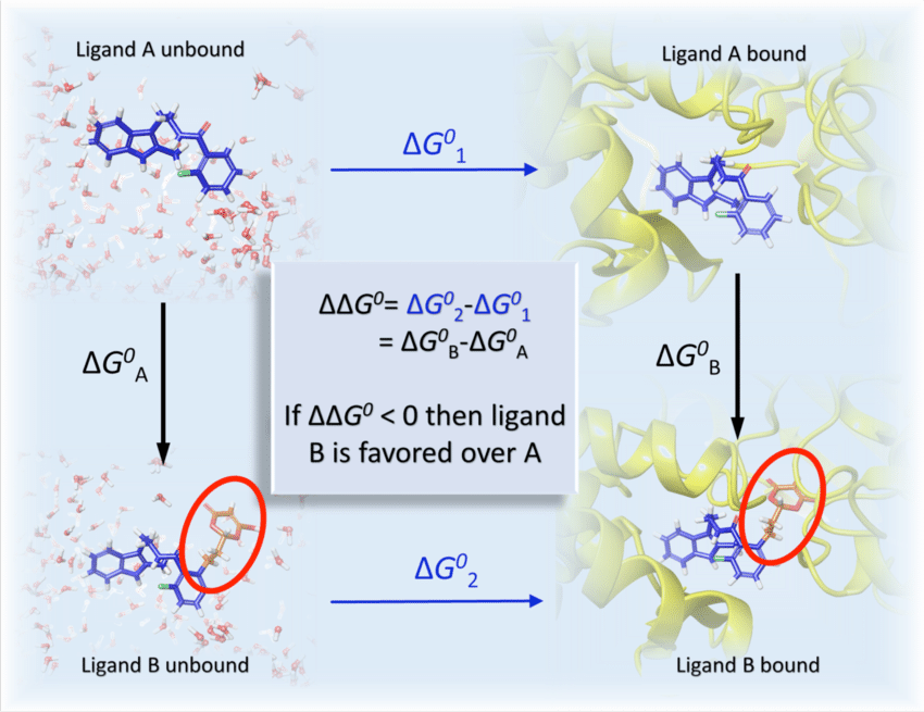
Figure 1: Thermodynamic cycle for RBFE calculations (source: JCAMD)
The key insight is that ΔΔG equals the difference between two “alchemical” transformations, where we morph one molecule into another, rather than two absolute binding calculations. These morphing simulations are much cheaper and more accurate than computing absolute energies directly:
$$\Delta\Delta G_{bind} = \Delta G_{bind}^{A} - \Delta G_{bind}^{B} = \Delta G_{A->B}^{bound} - \Delta G_{A->B}^{unbound} $$
Why “Alchemical”?
We call these calculations “alchemical” because we’re doing something impossible in the real world: gradually transforming one molecule into another inside the simulation. The atoms unique to molecule A are slowly “turned off” while the atoms unique to molecule B are “turned on”. This is controlled by a coupling parameter λ (lambda), the same approach used in ABFE: at λ = 0 molecule A is fully present; at λ = 1 molecule B is fully present; intermediate λ values describe a continuous, non-physical hybrid state.
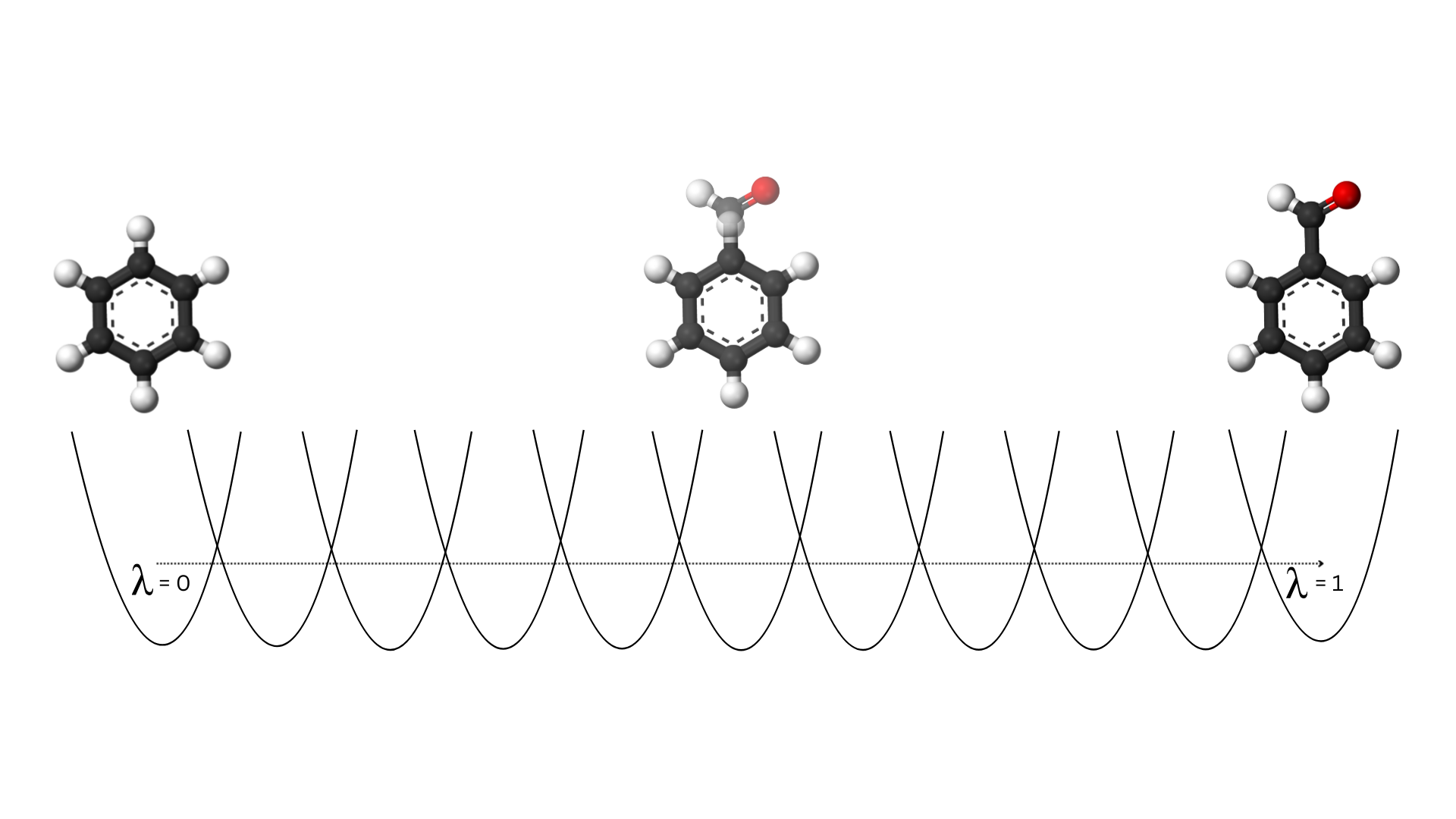
Figure 2: Alchemical transformation of benzene to benzaldehyde over 11 lambda states
Think of it like a movie dissolve effect, but for molecules. This continuous, controlled transformation lets us precisely measure the energy difference between the two states.
A technical subtlety is that as atoms appear or disappear at the endpoints (λ = 0 or λ = 1), standard Lennard-Jones potentials become singular — two atoms occupying the same space would produce infinite repulsion. Soft-core potentials solve this by smoothly switching on van der Waals interactions, preventing numerical instabilities at the transformation endpoints.
Building a Network
In practice, RBFE isn’t used to compare just two molecules; it’s used to screen many at once. Calculations are organized into a transformation network connecting all the molecules under study:
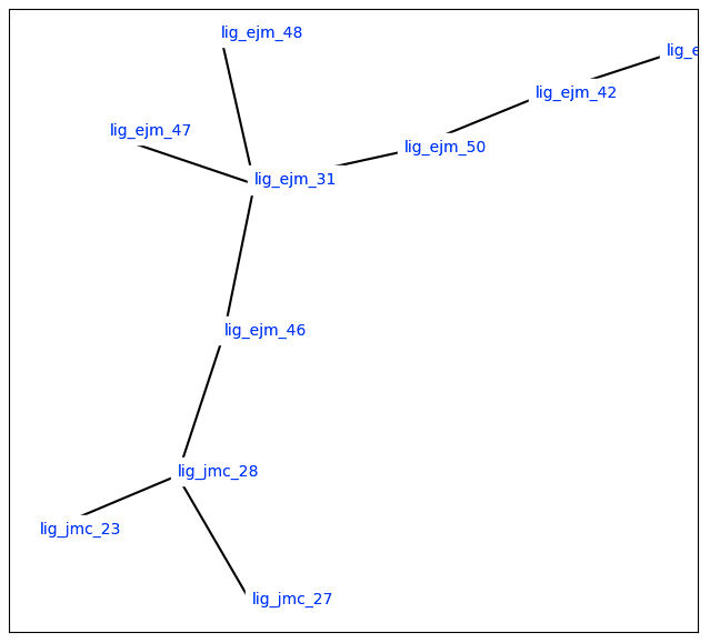
Figure 3: Minimal Spanning Tree for RBFE calculations (source: OpenFE)
Each edge in the network represents one transformation. By connecting molecules this way, we can:
- Cross-check results: If A→B = −1.0 kcal/mol and B→C = −0.5 kcal/mol, then A→C should be approximately −1.5 kcal/mol
- Minimize calculations: Only enough edges to connect the network are needed, not every pair
- Identify errors: Thermodynamic inconsistencies flag problematic calculations
Network Topologies
The structure of the network affects both accuracy and computational cost:
| Topology | Description | Best For |
|---|---|---|
| Minimal Spanning Tree (MST) | Fewest transformations to connect all molecules | Large compound sets, initial screening |
| Radial (Star) | All molecules transform to/from one reference | SAR studies around a lead compound |
| Maximal | All possible pairwise transformations | Maximum accuracy, small sets |
The Role of Atom Mapping
For each transformation to work, the simulation needs to know which atoms in molecule A correspond to which atoms in molecule B. This atom mapping determines what stays, what disappears, and what appears during the morph.
- Matching atoms remain unchanged throughout the transformation
- Atoms unique to A gradually disappear
- Atoms unique to B gradually appear
Kartograf is a 3D-aware atom mapper that considers both chemical similarity and spatial geometry to produce optimal mappings, which directly affects the accuracy of the result.
Interpreting the Results
RBFE results are reported as ΔΔG values in kcal/mol:
- Negative ΔΔG: The new molecule binds more strongly than the reference
- Positive ΔΔG: The new molecule binds more weakly than the reference
- Magnitude: Every 1.4 kcal/mol corresponds to roughly a 10-fold change in binding affinity
For example, a molecule with ΔΔG = −2.8 kcal/mol relative to the reference binds approximately 100× more tightly.
Accuracy and Limitations
Modern RBFE calculations typically achieve:
- Root-mean-square error: ~1.0 kcal/mol vs. experiment
- Correlation (R²): 0.5–0.8 with experimental data
- Best for: Similar molecules sharing a common scaffold — the core ring system or backbone shared by the series — with varied substituents around it
The method works best when molecules are structurally similar. Large scaffold changes, where the central ring system itself changes, or unusual chemistry can reduce reliability: in those cases, ABFE is the better choice. A rough decision guide:
| Situation | Recommended Method |
|---|---|
| Comparing similar analogues (same scaffold, different substituents) | RBFE |
| Evaluating a structurally novel compound | ABFE |
| Needing an absolute Kd or IC₅₀ prediction | ABFE |
| Ranking a large library of similar compounds | RBFE |
Common RBFE Implementation
Modern RBFE workflows typically use the OpenFE open-source ecosystem. The commercial equivalent, FEP+ from Schrödinger, follows the same theoretical principles but within a proprietary platform and is widely used in industry:
- Kartograf: 3D-aware atom mapper that considers both chemical similarity and spatial geometry to produce high-quality mappings
- OpenMM: GPU-accelerated molecular dynamics engine for running the λ-window simulations
- LOMAP (Lead Optimization Mapper): scores proposed transformations by similarity and suggests efficient network layouts, minimising the number of calculations needed to connect all compounds
- Hamiltonian Replica Exchange (HREX): enhanced sampling strategy where replicas at adjacent λ values periodically swap configurations, allowing the ligand to escape local minima and improving convergence of the free energy estimate
A typical workflow proceeds as:
- Prepare the protein structure and ligand series
- Select a network topology (MST is recommended for most cases)
- Review the proposed network and atom mappings
- Run calculations across all transformation edges
- Analyze results as a ranked list with uncertainty estimates
For understanding the electronic properties of the ligands themselves — charge distribution, reactivity, conformational preferences — quantum chemistry methods provide a complementary perspective that classical force fields cannot offer.
References
- Ries, B., et al. (2023). Kartograf: A Geometrically Accurate Atom Mapper for Hybrid-Topology Relative Free Energy Calculations. Journal of Chemical Theory and Computation. doi:10.1021/acs.jctc.3c01206
- Shirts, M. R., & Chodera, J. D. (2008). Statistically optimal analysis of samples from multiple equilibrium states. Journal of Chemical Physics, 129(12), 124105. doi:10.1063/1.2978177
- Cournia, Z., Allen, B., & Sherman, W. (2017). Relative Binding Free Energy Calculations in Drug Discovery: Recent Advances and Practical Considerations. Journal of Chemical Information and Modeling, 57(12), 2911–2937. doi:10.1021/acs.jcim.7b00564
- Eastman, P., et al. (2017). OpenMM 7: Rapid development of high performance algorithms for molecular dynamics. PLOS Computational Biology, 13(7), e1005659. doi:10.1371/journal.pcbi.1005659
- Wang, L., et al. (2015). Accurate and Reliable Prediction of Relative Ligand Binding Potency in Prospective Drug Discovery by Way of a Modern Free-Energy Calculation Protocol and Force Field. Journal of the American Chemical Society, 137(7), 2695–2703. doi:10.1021/ja512751q
- Schindler, C. E. M., et al. (2020). Large-Scale Assessment of Binding Free Energy Calculations in Active Drug Discovery Projects. Journal of Chemical Information and Modeling, 60(9), 4120–4130. doi:10.1021/acs.jcim.0c00900
- Loeffler, H. H., et al. (2018). Reproducibility of Free Energy Calculations across Different Molecular Simulation Software Packages. Journal of Chemical Theory and Computation, 14(11), 5567–5582. doi:10.1021/acs.jctc.8b00544
Konstantin N
BLOG
RBFE Free Energy Theory Drug Discovery