Theory
Absolute Binding Free Energy: Measuring Affinity In Silico
What is Absolute Binding Free Energy?
When a drug binds to a protein, it releases or absorbs energy. Absolute Binding Free Energy (ABFE) quantifies exactly how much: it is the Gibbs free energy difference between a ligand freely dissolved in water and that same ligand bound in the protein’s active site.
Unlike a simple enthalpy measurement, this free energy accounts for everything simultaneously: the direct interaction energy between protein and ligand, the energetic cost of displacing ordered water molecules from the binding pocket, and the entropy penalty the ligand pays by losing conformational and translational freedom upon binding. This single number, expressed as $ΔG$ in kcal/mol, is a more complete measure of binding strength than any individual energy component. A more negative $ΔG$ means stronger, tighter binding.
In contrast to Relative Binding Free Energy (RBFE), which measures the difference in affinity between two similar molecules, ABFE gives the actual value for a single compound, meaning it can be used in cases where
- You have a single promising compound and need to know its true potency
- You want to predict experimental $IC_{50}$ or $K_d$ values directly
- You’re deciding whether a computational hit is worth pursuing experimentally
The Thermodynamic Cycle
Direct simulation of a ligand binding to a protein is computationally intractable; the spontaneous binding event would take years to observe. Instead, ABFE uses a thermodynamic cycle built on “alchemical” transformations.
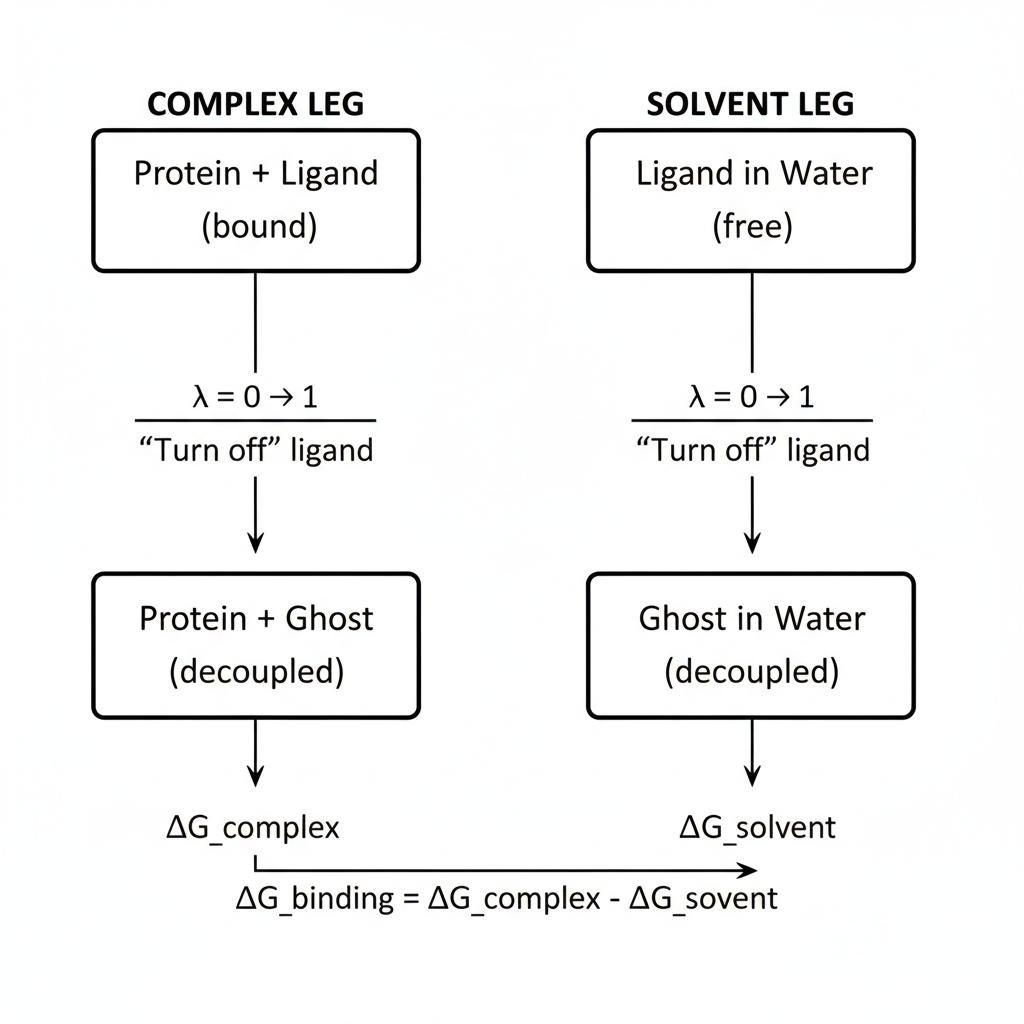
Figure 1: Thermodynamic cycle for ABFE calculations
Since free energy is a state function, the path doesn’t matter, only the endpoints. We therefore run two independent sets of simulations, each gradually annihilating the ligand from a different starting environment:
- $ΔG_{complex}$: the ligand starts bound in the protein pocket and is decoupled from all surrounding atoms as λ increases from 0 to 1. This leg measures how strongly the protein holds onto the ligand.
- $ΔG_{solvent}$: the ligand starts freely solvated in bulk water and the same decoupling is applied, measuring how much energy is required to remove the ligand from solvent.
The binding free energy follows directly from the difference: $$ΔG_{bind} = ΔG_{complex} − ΔG_{solvent}$$
Alchemical Transformations
To compute these annihilation energies, simulations gradually “turn off” the ligand by scaling its interactions with the environment. This is controlled by a coupling parameter λ (lambda):
- $λ = 0$: ligand is fully present and interacting normally
- $λ = 0.5$: ligand interactions are at half-strength (a non-physical, intermediate state)
- $λ = 1$: ligand is completely decoupled, invisible to its surroundings
The annihilation is performed in two stages. First, the partial charges on the ligand are switched off; this removes electrostatic interactions. Then, the van der Waals interactions (described by the Lennard-Jones potential) are gradually switched off. This order is important: removing van der Waals before charges would create unphysical “charged ghosts”, atoms that interact electrostatically but pass through matter, which destabilises the simulation.
By running separate simulations across many λ values (typically 11–20 “windows”), we map out the energy change along the entire transformation pathway and integrate to obtain $ΔG$
The complex leg is more complicated and will take longer to execute as there are more atoms in the system. Furthermore, once the ligand is fully decoupled at $λ = 1$, it no longer feels the protein and can drift to any position in the simulation box. This would introduce an enormous and artificial translational entropy contribution, therefore, harmonic restraints are applied on the ligand’s position and orientation relative to the protein and corrected for analytically - a methodology formalized by Boresch et al.
Enhanced Sampling with Replica Exchange
A key challenge in free energy calculations is ensuring each simulation adequately explores the relevant conformational space. Modern ABFE protocols address this with Hamiltonian Replica Exchange (HREX):
- Multiple copies (replicas) of the system run simultaneously at different λ values
- Neighboring replicas periodically attempt to swap configurations
- Swapping allows conformational states to propagate across the λ series, escaping local minima
- The result is faster convergence and more reliable free energy estimates
Accuracy and Computational Cost
ABFE is computationally demanding but highly accurate relative to other computational methods:
| Aspect | Typical Value |
|---|---|
| Accuracy vs. experiment | ~1–2 kcal/mol error |
| Wall-clock time | Hours to days on GPU hardware |
| Applicability | Any ligand–protein pair |
Because no structural similarity between ligands is required, ABFE is more broadly applicable than RBFE—though this generality comes at greater computational expense.
Interpreting the Results
A complete ABFE calculation produces several outputs worth examining:
- $ΔG_{bind}$: The final binding free energy estimate
- Statistical uncertainty: Error bars from MBAR (Multistate Bennett Acceptance Ratio) analysis. MBAR is a statistically optimal method that combines information from all λ windows simultaneously to produce the most accurate possible free energy estimate from the available data
- Overlap matrices: Quantify how much the phase-space sampled by adjacent λ windows overlaps. Sufficient overlap is required for MBAR to produce a reliable estimate; poor overlap between neighbouring windows indicates that additional intermediate λ values are needed
- Convergence plots: Show how the $ΔG$ estimate evolves as a function of simulation time. A converged calculation should show a stable, flat estimate in the second half of the simulation
- Replica exchange acceptance rates: Indicate how effectively configurations are mixing between λ windows; rates of 20–40% are typically desirable
Results are reported as $ΔG$ in kcal/mol. The table below gives a rough sense of how these values relate to experimentally measurable binding constants:
| $ΔG$ (kcal/mol) | Approximate $K_d$ | Binding Strength |
|---|---|---|
| −6 | 40 μM | Weak |
| −8 | 1 μM | Moderate |
| −10 | 50 nM | Strong |
| −12 | 1 nM | Very strong |
The conversion follows: $K_d = exp(ΔG / RT)$, where $RT ≈ 0.6 kcal/mol$ at 298 K.
References
- Mobley, D. L., & Gilson, M. K. (2017). Predicting Binding Free Energies: Frontiers and Benchmarks. Annual Review of Biophysics, 46, 531–558. doi:10.1146/annurev-biophys-070816-033654
- Shirts, M. R., & Chodera, J. D. (2008). Statistically optimal analysis of samples from multiple equilibrium states. Journal of Chemical Physics, 129(12), 124105. doi:10.1063/1.2978177
- Eastman, P., et al. (2017). OpenMM 7: Rapid development of high performance algorithms for molecular dynamics. PLOS Computational Biology, 13(7), e1005659. doi:10.1371/journal.pcbi.1005659
- Hahn, D. F., et al. (2022). Best Practices for Constructing, Preparing, and Evaluating Protein-Ligand Binding Affinity Benchmarks. Living Journal of Computational Molecular Science, 4(1), 1497. doi:10.33011/livecoms.4.1.1497
- Boresch, S., Tettinger, F., Loebl, M., & Karplus, M. (2003). Absolute Binding Free Energies: A Quantitative Approach for Their Calculation. Journal of Physical Chemistry B, 107(35), 9535–9551. doi:10.1021/jp0217839
- Klimovich, P. V., Shirts, M. R., & Mobley, D. L. (2015). Guidelines for the analysis of free energy calculations. Journal of Computer-Aided Molecular Design, 29(5), 397–411. doi:10.1007/s10822-015-9840-9
Konstantin N
BLOG
ABFE Free Energy Theory Drug Discovery